K-means Clustering Using Stocks Data
Introduction
Through the use of data mining technology, large amounts of complex financial data can be analyzed. K-means clustering (KMC) is an algorithm that can be used for potentially maximizing profit, or reducing risk, when investing in company stocks or indexes (Momeni, Mohseni, and Soofi 2015). Using KMC, stock data can be grouped together in accordance with predetermined criteria to find similarity, dissimilarity, and structure. KMC can also be used to classify financial features according to maximum and minimum similarity (Zuhroh, Rofik, and Echchabi 2021). Clustering algorithms, such as the K-means clustering (KMC) algorithm, have gained attention as valuable tools for aiding investment decision-making. However, there are some shortcomings to the method including the determination of the number of ‘k clusters’, different distance calculation methods, and the problem of local extremum (Fang and Chiao 2021).
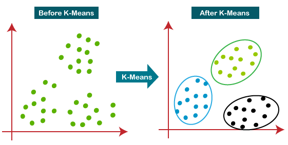
KMC is a version of unsupervised machine learning utilizing algorithms to analyze and cluster datasets that are unlabeled (Malik and Tuckfield 2019). In this case, K-means clustering would be considered an unsupervised learning method where similar data points will be assembled into groups of unlabeled data . It groups similar unlabled data by looking at the average distance between the objects in each group which is known as the centroid and the K groups. (“Figure 1: KMC Algorith,” n.d.) below shows a visual representation of k-means. K-means measures the distance between each objects and centroid and is then assigned to the correct groups until all objects have a group (Yuan and Yang 2019). In order to weigh variables one process that can be used is the ‘Analytic Hierarchal Process’. The stages of the KMC algorithm were as follows:
Initial stage that partitioned the objects randomly into ‘k’ clusters.
The repetition stage by calculating the center of each cluster using the mean of the data, compute the squared Euclidean distance from each object to each cluster, and compute the squared error function.
The improvement stage where objects were assigned to the cluster with the nearest center.
The stop stage which was a process that continued until no object move clusters or the objective function value doesn’t reduce (Momeni, Mohseni, and Soofi 2015).
Stocks data can be predicted using both qualititative and quantitative company information, some studies discovered that qualitative information does a better job at predicting stocks. Qualitative data uses information such as how the company performs versus quantitative data using numbers such as a company assets (Babu, Geethanjali, and Satyanarayana 2012). Using KMC it can help stock buyers or sellers understand the stock market pattern. K-means clustering when combined with regression method also helps with predicting stock future stock prices. This allows users to know when the best time to get in the market before a price increase/decrease, which in turn, tells sellers to hold or to sell their stocks (Bini and Mathew 2016). KMC does have limitations including the determination of the number of ‘k clusters’, different distance calculation methods, and the problem of local extremum (Fang and Chiao 2021). Other types of limitations include the inability to use all types of data with KMC (Ahmed, Seraj, and Islam 2020).
Due to some of the limitations of KMC, we also reviewed some proposed improvements. One of the proposed resolution is the fact that there is a need for better initial centroids, and the way to do so is by sorting the data points distance-wise and separating them into equal sets. By partitioning the data in a sorted method leads to better results. The authors then reassign the data points to the correct clusters by looking at the distance between the centroid to whichever cluster is closest (Yedla, Pathakota, and Srinivasa 2010). The time complexity involved with k-means clustering was also addressed. The proposed method uses a heap sort method, which is O(nlogn); combining that with the time complexity, we still see that time complexity is O(nlogn) on average. This confirms that the proposed method in this article is more efficient than the original k-means clustering. The experimental results also corroborate this. This paper provides an overview of KMC, some of the limitations of the methodology, improvements, as well as our analysis on how well KMC does handling stock data.
Methods
There are several methods involved when selecting the optimal number of clusters. This paper we considered the elbow, silhouette, and gap statistics method.
The Elbow Method is used to find a good number of cluster by looking at a point where the sum of squares error (SSE) decreases rapidly. SSE looks at how far each point is from the center of its cluster, essentially the points should be close together to minimize the SSE (Yuan and Yang 2019).
Steps to find the best cluster number using elbow method:
Select different number of clusters to try
Calculate the SSE for each cluster
Plot the SSE on the x axis number of clusters, while on the y axis will show the SSE
Once you plot the results will show in an elbow shape, the point found in the elbow shows SSE decreasing rapidly. That point is considered the optimal cluster number.
Silhouette Method - The Silhouette method is used to determine how well data points fits into their cluster. It does so by looking at how close the data point is to its own cluster compared to the other clusters (Ossareh, Pourjafar, and Kopczewski 2021).
Gap Statistic Method - The Gap Statistic method is used to find the k value with the largest gap to help compare the within-cluster dispersion. Using this method along with the other 2 we can determine which is best to select the optimal cluster number. \[ G(k) = E_n(\log(W_k)) - \log(W_k) \]
\[ W_k = \frac{1}{P} \sum_{b=1}^{P} \log(W^*_{kb}) \approx \frac{1}{P} \sum_{b=1}^{P} \log(W^*_{kb}) \]
Euclidean Distance
Calculating the distance for KMC can be achieved by a few different method. By default Euclidean distance, is used to calculate the distance between a point and it’s initial cluster (Yedla, Pathakota, and Srinivasa 2010). The Euclidean distance uses the Pythagorean theorem; however, not only in two dimensions, but with as many dimensions as needed.
\[ d_{euc}(x, y) = \sqrt{\sum_{i = 1}^{n}{(x_i - y_i)^2}} \] K-means Without Time Series Analysis
K-means was used as a pattern clustering technique to gain important information related to the stock market- specifically the S&P 500. Using the clustering algorithm, associated metrics are grouped together in subsets to analyze and build portfolios (Nanda, Mahanty, and Tiwari 2010). Time series does NOT have to be used in the analysis; instead, returns for varying periods can be used such as for short term: 1 day, 1 week, 30 days; or long term such as 3 months, 6 months, or 1 year (Nanda, Mahanty, and Tiwari 2010). For this paper, returns where considered on a monthly basis (short term).
Analysis and Results
The dataset was taken from the publication “Irrational Exuberance” by Robert Shiller (Shiller 2015). The dataset summarized 150 years of data on the S&P 500 index which consisted of the 500 largest companies by market capitalization listed on stock exchanges in the United States (“S&P 500 SPX 500,” n.d.). Specifically, the dataset metrics included the S&P 500 composite index valuation, dividends, earnings, consumer price index, long interest rate, real price, real dividend, real total price, real earnings, cyclically adjusted price earnings ratio, monthly total bond returns, and others. For the project’s analysis, the data was converted to month-by-month percentage changes to make meaningful clusters which included the composite index, consumer price index, long-term interest rates, real earnings, cyclically adjusted price to earnings ratio (adjusted and total), and real total bond return. The dataset was limited to the years 2012 to present considering that more recent data may be more germane to today’s dynamic market conditions. The CAPE ratio was included in the dataset which was an innovative metric proposed by Robert Shiller which is calculated as follows (Shiller 2015). \[ \text{Cyclically adjusted price - to - earnings ratio} = \frac{\text{Share Price}}{{\text{(10-year Inflation Adjusted Average Earnings)}}} \] The CAPE ratio has the purported advantage of measuring valuation over a ten-year period to smooth out random fluctuations in corporate profits thereby providing an effective forecasting tool to identify undervalued or overvalued indexes or stocks. The historical average of the CAPE ratio for the S&P 500 has been 16.8; however, climbing ratios of 28 starting in 1997 accurately predicted the dotcom bubble crash of 2000 followed by the prediction of the 2008 market crash. Although some critics point out limitations of the CAPE ratio being too backward looking; market bubbles and unrealistic equity returns using CAPE have been accurately predicted.
Data and Visualization
The packages relevant to the project that were needed included factoextra(), NbClust(), and Cluster(). For example, factoextra can run the k-means algorithm along with visualizations. Also, NbClust() and Cluster() can assist in determining the optimal number of clusters and centroids.
Code
# loading packages
library(readr)
library(tidyverse)
library(ggplot2)
library(cluster)
library(NbClust)
library(factoextra)
library("dplyr")
library(gridExtra)
library(knitr)
# read csv file into R
df<- read_csv("SPDatasetLAST.csv")
#view the data headers
head(df)
# A tibble: 6 × 7
SPCompIndexPercentChange CPIPercentChange LongInterestRatePercentChange
<dbl> <dbl> <dbl>
1 0.04 0.00296 0.110
2 0.02 0.00821 0.0366
3 0.02 0.00258 -0.0101
4 0.01 -0.00103 -0.102
5 0.04 0.00181 0.0966
6 -0.01 0.00236 0.192
# ℹ 4 more variables: RealEarningsPercentChange <dbl>,
# CyclicallyAdjPEPercentageChange <dbl>, CAPETotalPercentageChange <dbl>,
# RealTotalBondReturnPercentageChange <dbl>Scale() assists with standardizing the data so that it is comparable using “z-scores”.
Code
# standardize the data having a standard normal with a mean of 0 and a standard deviation of 1
df<-scale(df)
#view the data
head(df)
SPCompIndexPercentChange CPIPercentChange LongInterestRatePercentChange
[1,] 0.89659338 0.20265878 1.0060604
[2,] 0.33961870 1.65299283 0.2579556
[3,] 0.33961870 0.09832691 -0.2158457
[4,] 0.06113137 -0.90124837 -1.1476315
[5,] 0.89659338 -0.11679980 0.8654489
[6,] -0.49584331 0.03659162 1.8294544
RealEarningsPercentChange CyclicallyAdjPEPercentageChange
[1,] -0.08698395 0.8407465
[2,] -0.28180011 0.1198802
[3,] -0.07361572 0.4154007
[4,] 0.36261716 0.1549720
[5,] 0.24822909 0.9826116
[6,] 0.21833802 -0.6941067
CAPETotalPercentageChange RealTotalBondReturnPercentageChange
[1,] 0.8474031 -0.9274587
[2,] 0.1423810 -0.6077692
[3,] 0.4217869 0.1363896
[4,] 0.1611393 1.2431075
[5,] 0.9936749 -0.7642882
[6,] -0.6890358 -1.7469219Code
kable(head(df))| SPCompIndexPercentChange | CPIPercentChange | LongInterestRatePercentChange | RealEarningsPercentChange | CyclicallyAdjPEPercentageChange | CAPETotalPercentageChange | RealTotalBondReturnPercentageChange |
|---|---|---|---|---|---|---|
| 0.8965934 | 0.2026588 | 1.0060604 | -0.0869839 | 0.8407465 | 0.8474031 | -0.9274587 |
| 0.3396187 | 1.6529928 | 0.2579556 | -0.2818001 | 0.1198802 | 0.1423810 | -0.6077692 |
| 0.3396187 | 0.0983269 | -0.2158457 | -0.0736157 | 0.4154007 | 0.4217869 | 0.1363896 |
| 0.0611314 | -0.9012484 | -1.1476315 | 0.3626172 | 0.1549720 | 0.1611393 | 1.2431075 |
| 0.8965934 | -0.1167998 | 0.8654489 | 0.2482291 | 0.9826116 | 0.9936749 | -0.7642882 |
| -0.4958433 | 0.0365916 | 1.8294544 | 0.2183380 | -0.6941067 | -0.6890358 | -1.7469219 |
The Elbow method was used to help determine the optimal number of clusters using the coded algorithm fviz_nbclust(). The elbow method used an unsupervised algorithm approach from a calculation known as the within-cluster sum of squares (WCSS) method.
Code
#estimate the optimal number of clusters according to the number of bends (elbow method)
fviz_nbclust(df, kmeans, method = "wss") +
    geom_vline(xintercept = 4, linetype = 2)+
  labs(subtitle = "Elbow method")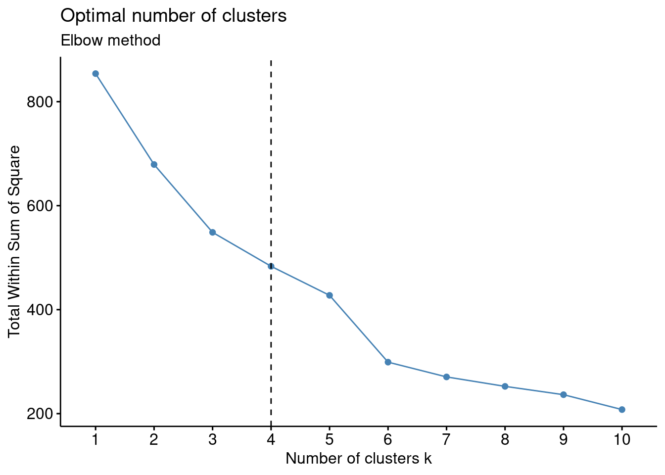
The Silhouette method is an unsupervised method to determine the optimum number of clusters. It uses a mathematical formula to measure how well a data point fits within a cluster through the Silhouette coefficient.
Code
#estimate the optimal number of clusters Silhouette method
fviz_nbclust(df, kmeans, method = "silhouette")+
  labs(subtitle = "Silhouette method")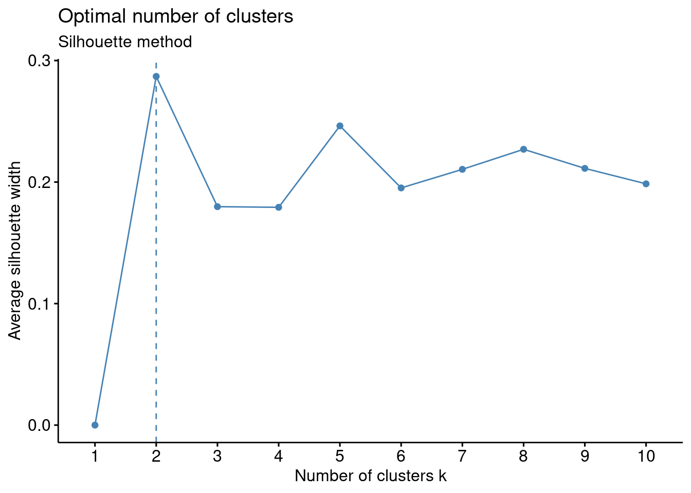
The “Gap statistic method” is another algorithm that can be used to identify the optimum number of clusters. The method standardizes the data using a logarithmic function.
Code
#estimate the optimal number of clusters with the 'gap statistics' method
fviz_nbclust(df, kmeans, nstart = 25,  method = "gap_stat", nboot = 50)+
  labs(subtitle = "Gap statistic method")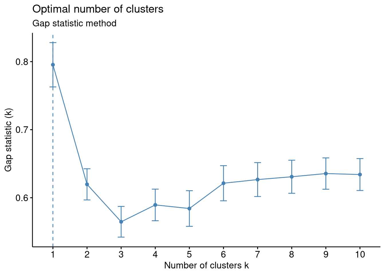
The coded algorithm NbClust() uses 30 different methods to help determine the optimal number of clusters. The selected distance method was “Euclidean” which uses essentially Pythagorean theorem to find the relative distances between the data points.
Code
#NbClust provides 30 indexes for determining the optimal number of clusters in a data set and offers the best clustering scheme from different results
nb <- NbClust(df, distance = "euclidean", min.nc = 2,
        max.nc = 10, method = "kmeans")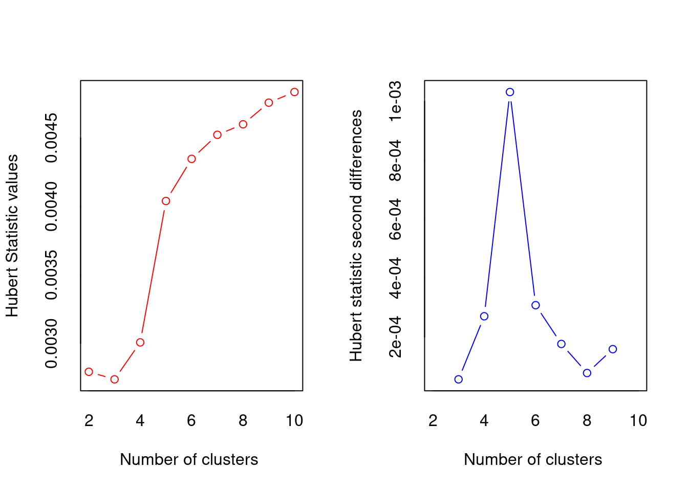
*** : The Hubert index is a graphical method of determining the number of clusters.
                In the plot of Hubert index, we seek a significant knee that corresponds to a
                significant increase of the value of the measure i.e the significant peak in Hubert
                index second differences plot.
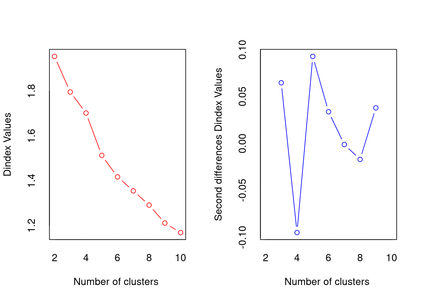
*** : The D index is a graphical method of determining the number of clusters.
                In the plot of D index, we seek a significant knee (the significant peak in Dindex
                second differences plot) that corresponds to a significant increase of the value of
                the measure.

*******************************************************************
* Among all indices:
* 6 proposed 2 as the best number of clusters
* 2 proposed 3 as the best number of clusters
* 3 proposed 4 as the best number of clusters
* 6 proposed 5 as the best number of clusters
* 2 proposed 6 as the best number of clusters
* 1 proposed 7 as the best number of clusters
* 1 proposed 9 as the best number of clusters
* 3 proposed 10 as the best number of clusters

                   ***** Conclusion *****

* According to the majority rule, the best number of clusters is  2


*******************************************************************
The K-means algorithm coding: “K-means()” was used for differing number of centroids (k=3 through k=6) and analyzed for relevance.
Code
#test kmeans cluster for k=3, k=4 and k=5 for comparison
k3 <- kmeans(df, centers = 3, nstart = 25)
k4 <- kmeans(df, centers = 4, nstart = 25)
k5 <- kmeans(df, centers = 5, nstart = 25)
k6 <- kmeans(df, centers = 6, nstart = 25)
The coded algorithm fviz_cluster() plots the clusters using the selected number of centroids. In this case, k=3 through k=6.
Code
# plots to compare
p1 <- fviz_cluster(k3, geom = "point", data = df) + ggtitle("k = 3")
p2 <- fviz_cluster(k4, geom = "point",  data = df) + ggtitle("k = 4")
p3 <- fviz_cluster(k5, geom = "point",  data = df) + ggtitle("k = 5")
p4 <- fviz_cluster(k6, geom = "point",  data = df) + ggtitle("k = 6")
grid.arrange(p1, p2, p3, p4, nrow = 2)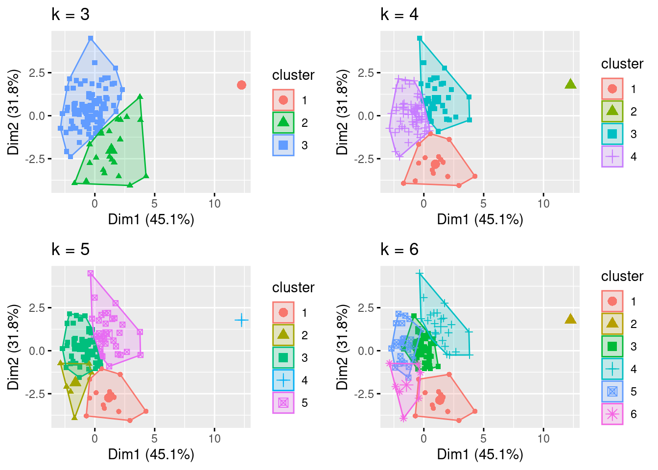
The output of K-means() was assigned to different data frames (final3 through final6) for further analyses and selection of the optimal number of clusters.
Code
#Cluster analysis, k=3, nstart = 25 will generate 25 initial configurations
set.seed(123)
final3 <- kmeans(df, 3, nstart = 25)
final4 <- kmeans(df, 4, nstart = 25)
final5 <- kmeans(df, 5, nstart = 25)
final6 <- kmeans(df, 6, nstart = 25)
Based on the analysis of the output data and visualizations, k=4 was selected and the results are displayed using the print().
Code
#view the kmeans clustering including: cluster, centers, total sum of squares, vector of within-cluster sum squares, total within-sum of squares, the between-cluster sum of squares, and number of points in each cluster
print(final4)
K-means clustering with 4 clusters of sizes 69, 1, 38, 15
Cluster means:
SPCompIndexPercentChange CPIPercentChange LongInterestRatePercentChange
1 0.5091327 0.04409966 0.1741670
2 -6.9010521 -1.21471372 -4.3700644
3 -0.3859141 -0.53345867 -0.7321102
4 -0.9042914 1.22955111 1.3448485
RealEarningsPercentChange CyclicallyAdjPEPercentageChange
1 0.1963760 0.5410223
2 -2.4270359 -5.8070446
3 -0.2155105 -0.3902915
4 -0.1955674 -1.1128277
CAPETotalPercentageChange RealTotalBondReturnPercentageChange
1 0.5399368 -0.1757434
2 -5.7976262 3.5727109
3 -0.3852076 0.8583392
4 -1.1213416 -1.6042206
Clustering vector:
[1] 1 1 1 3 1 4 1 1 1 3 1 1 1 3 1 3 3 1 3 3 1 3 1 3 3 1 1 3 4 4 3 3 3 1 1 3 3
[38] 3 1 1 3 3 1 1 1 1 1 1 1 1 1 3 1 1 1 3 1 1 1 1 1 4 3 3 1 1 1 1 1 4 3 3 3 1
[75] 1 1 3 3 3 3 1 3 1 1 1 3 2 3 1 1 1 1 3 1 1 1 1 1 4 1 1 1 1 1 1 4 1 3 4 4 4
[112] 4 4 4 3 1 4 4 1 3 1 1 3
Within cluster sum of squares by cluster:
[1] 225.55854 0.00000 115.11444 77.20815
(between_SS / total_SS = 51.1 %)
Available components:
[1] "cluster" "centers" "totss" "withinss" "tot.withinss"
[6] "betweenss" "size" "iter" "ifault" The analysis made use of several R packages including the following:
• The ‘NbClust’ package assisted in cluster analysis by finding the optimal number of groups in the data (Maechler, 2023).
• The “factoextra” package was used to calculate and visualize kmeans (Kassambara and Mundt 2023).
The entire dataset included metrics that generated clusters that were not meaningful considering the expected result in terms of S&P 500 index returns versus economic and corporate data. Therefore, several trials were conducted until meaningful results and clusters were generated. The data was ‘normalized’ using scale() to allow for comparable data using z-score versus raw data. Determining the optimal number of clusters considering the various methods returned inconsistent including Elbow method: 4 clusters, Silhouette method: 2, Gap statistic: 1, Humbert statistic: 5, D index: 4, and other proposed indices. Considering the lack of agreement in the optimal number of clusters, the visualizations were analyzed as were the cluster means. The visualization with k=4 provided well-defined clusters with minimal overlap. However, k=5 and k=6 visualizations had poorly defined clusters with significant overlap (Géron 2022). Additionally, the distance of the data from the centroids for cluster with k=4 visually appeared sufficiently small. The elbow method corresponded with k=4 where a ‘bend’ in the data was identified with four clusters. Also, the Dunn index indicated four clusters; this metric sets to identify clusters that are the most compact and well separated. Additionally, the cluster means data was analyzed for k=3, k=4, k-5, and k=6 considering the expected results given economic and corporate indicators and movements in the S&P 500 index. It was therefore determined that k=4 was the optimal number of clusters with sizes of 69, 1, 38, and 15. Although one cluster had only “1” data point, it was not eliminated as an outlier since stock market traders are faced with extreme events in the stock market, and these shocks should not be ignored considering significant shifts can severely affect portfolios. In this context, extreme events that become predictable using kmeans may be useful to traders.
Statistical Modeling
The kmeans centroids delivered results that would be expected as follows:
• Cluster 1: the moderate increase of the S&P 500 of this cluster mean was ≈ 0.51 which was clustered with a slight increase in consumer price index ≈ 0.04 (a metric to reflect inflation), a small increase in long interest rate ≈ 0.17 (this often occurs when the Federal Reserve responds to increasing inflation with interest rate increases often correlated to increasing stock market pricing), a small increase in real earnings ≈ 0.20, a significant increase in CAPE ≈ 0.54 (a positive predictor for market valuation increase), and a small decrease in total bond return ≈ -0.18 (investors often move assets out of fixed income into stocks when stock market returns are deemed favorable) (Bosco and Khan 2018)
• Cluster 2: only contained one data point showing a nearly 7 standard deviation decrease from the mean indicating a market crash which was clustered with a significant decrease in consumer price index (deflation), a significant decrease in long interest rates (the Federal Reserve rapidly cutting interest rates), a significant decrease in real earnings and CAPE, while total bond returns significantly increased (consistent with traders moving money out of a crashing stock market into the safe haven of bonds) (Bosco and Khan 2018).
• Cluster 3: a moderate decline in the stock market ≈ -0.39 was clustered with moderate deflation, real earnings loss, a CAPE decrease, and a moderate return in bonds.
• Cluster 4: a significant decline in the stock market ≈ -0.90 was clustered with a significant increase in consumer price index ≈ 1.23 (inflation), a significant long interest rate increase ≈ 1.34, a small decline in real earnings ≈ -0.20, a significant decline in CAPE ≈ -1.12, and a significant decline in total bond return of ≈ -1.60.
The cluster means provided correlating metrics that a trader could potentially use to reap better gains when investing in the S&P 500. For example, both inflationary and deflationary cycles led to stock market losses (Bosco and Khan 2018). These losses were also reflected in the CAPE ratios. Stock market increases were correlated with insignificant inflationary pressures correlated with earnings increases and a positive CAPE. Traders could potentially use all of these factors as signals of when to buy and sell the S&P 500 thereby watching long interest rate, consumer price index, earnings, bond returns, and CAPE ratios to optimize the purchase and sale of the S&P 500 index demonstrating the utility of kmeans analysis.
Conclusion
For stock market traders and speculators, predicting market moves within the S&P 500 can significantly improve portfolio performance. Although there are many statistical methods that can assist in identifying buy and sell signals within the stock market, the K-means unsupervised learning algorithm can be helpful in recognizing metrics that traders can consider when managing their portfolio. Of the metrics available from the dataset, it was concluded that the composite index, consumer price index, long-term interest rates, real earnings, cyclically adjusted price to earnings ratio (adjusted and total), and real total bond return were the most germane in the context of K-means clustering. Determining the optimum number of clusters was difficult due to an inconsistency amongst the various clustering algorithms; therefore, a combination of visualization, results from the algorithms, and an understanding of market trends and predictions assisted in concluding that 4 clusters was the ideal. The results demonstrated that changes in the S&P 500 composite index moved in correlation with corporate earnings and price changes as well as macroeconomic indicators as expected based on market past performance and economic theory. Therefore, a speculator should take into consideration the aforementioned metrics identified through K-means when determining buy and sell triggers as it relates to the S&P 500 index of stocks.
References
Ahmed, Mohiuddin, Raihan Seraj, and Syed Mohammed Shamsul Islam. 2020. “The k-Means Algorithm: A Comprehensive Survey and Performance Evaluation.” Electronics 9 (8): 1295.
Babu, M Suresh, N Geethanjali, and B Satyanarayana. 2012. “Clustering Approach to Stock Market Prediction.” International Journal of Advanced Networking and Applications 3 (4): 1281.
Bini, BS, and Tessy Mathew. 2016. “Clustering and Regression Techniques for Stock Prediction.” Procedia Technology 24: 1248–55.
Bosco, Joish, and Fateh Khan. 2018. Stock Market Prediction and Efficiency Analysis Using Recurrent Neural Network. Grin Verlag.
Fang, Zheng, and Chaoshin Chiao. 2021. “Research on Prediction and Recommendation of Financial Stocks Based on k-Means Clustering Algorithm Optimization.” Journal of Computational Methods in Sciences and Engineering 21 (5): 1081–89.
“Figure 1: KMC Algorith.” n.d. https://www.javatpoint.com/k-means-clustering-algorithm-in-machine-learning.
Géron, Aurélien. 2022. Hands-on Machine Learning with Scikit-Learn, Keras, and TensorFlow. " O’Reilly Media, Inc.".
Kassambara, A, and F Mundt. 2023. “Factoextra: Extract and Visualize the Results of Multivariate Data Analyses. R Package Version 1.0. 7. The Comprehensive r Archive Network.”
Malik, Alok, and Bradford Tuckfield. 2019. Applied Unsupervised Learning with r: Uncover Hidden Relationships and Patterns with k-Means Clustering, Hierarchical Clustering, and PCA. Packt Publishing Ltd.
Momeni, Mansoor, Maryam Mohseni, and Mansour Soofi. 2015. “Clustering Stock Market Companies via k-Means Algorithm.” Kuwait Chapter of Arabian Journal of Business and Management Review 33 (2578): 1–10.
Nanda, SR, Biswajit Mahanty, and MK Tiwari. 2010. “Clustering Indian Stock Market Data for Portfolio Management.” Expert Systems with Applications 37 (12): 8793–98.
Ossareh, Adele, Mohammad Saeed Pourjafar, and Tomasz Kopczewski. 2021. “Cognitive Biases on the Iran Stock Exchange: Unsupervised Learning Approach to Examining Feature Bundles in Investors’ Portfolios.” Applied Sciences 11 (22): 10916.
Shiller, Robert J. 2015. “Irrational Exuberance.” In Irrational Exuberance. Princeton university press.
“S&P 500 SPX 500.” n.d. https://www.spglobal.com/spdji/en/indices/equity/sp-500/#overview.
Yedla, Madhu, Srinivasa Rao Pathakota, and TM Srinivasa. 2010. “Enhancing k-Means Clustering Algorithm with Improved Initial Center.” International Journal of Computer Science and Information Technologies 1 (2): 121–25.
Yuan, Chunhui, and Haitao Yang. 2019. “Research on k-Value Selection Method of k-Means Clustering Algorithm.” J 2 (2): 226–35.
Zuhroh, Idah, Mochamad Rofik, and Abdelghani Echchabi. 2021. “Banking Stock Price Movement and Macroeconomic Indicators: K-Means Clustering Approach.” Cogent Business & Management 8 (1): 1980247.