# A tibble: 6 × 7
  SPCompIndexPercentChange CPIPercentChange LongInterestRatePercentChange
                     <dbl>            <dbl>                         <dbl>
1                     0.04          0.00296                        0.110
2                     0.02          0.00821                        0.0366
3                     0.02          0.00258                       -0.0101
4                     0.01         -0.00103                       -0.102
5                     0.04          0.00181                        0.0966
6                    -0.01          0.00236                        0.192
# ℹ 4 more variables: RealEarningsPercentChange <dbl>,
#   CyclicallyAdjPEPercentageChange <dbl>, CAPETotalPercentageChange <dbl>,
# RealTotalBondReturnPercentageChange <dbl>K-means Clustering Using Stocks Data
2023-08-01
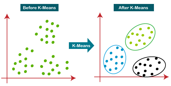
K-Means Process
1. Initial stage that partitioned the objects randomly into ‘k’ clusters.
2. The repetition stage by calculating the center of each cluster using the mean of the data, compute the squared Euclidean distance from each object to each cluster, and compute the squared error function.
3. The improvement stage where objects were assigned to the cluster with the nearest center.
4. The stop stage which was a process that continued until no object move clusters or the objective function value doesn’t reduce.
K-Means Cluster
Data and Visualization (Methods)
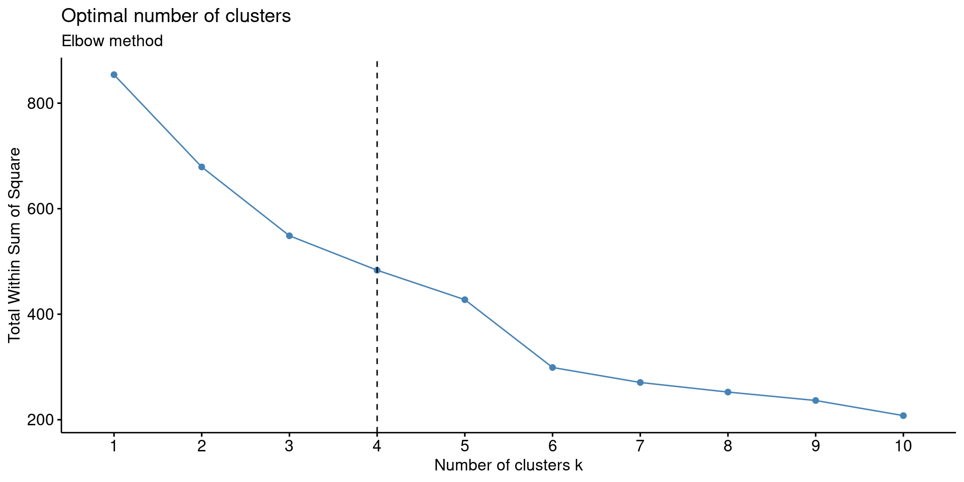
- Elbow Method to determine the optimal number of clusters using fviz_nbclust().
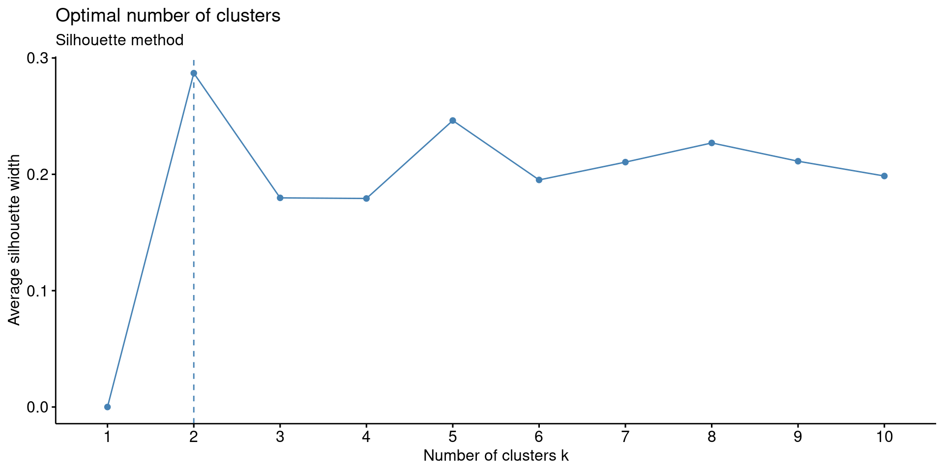
- Silhouette Method to determine the optimum number of clusters; it measures how well a data point fits within a cluster using the Silhouette Coefficient.
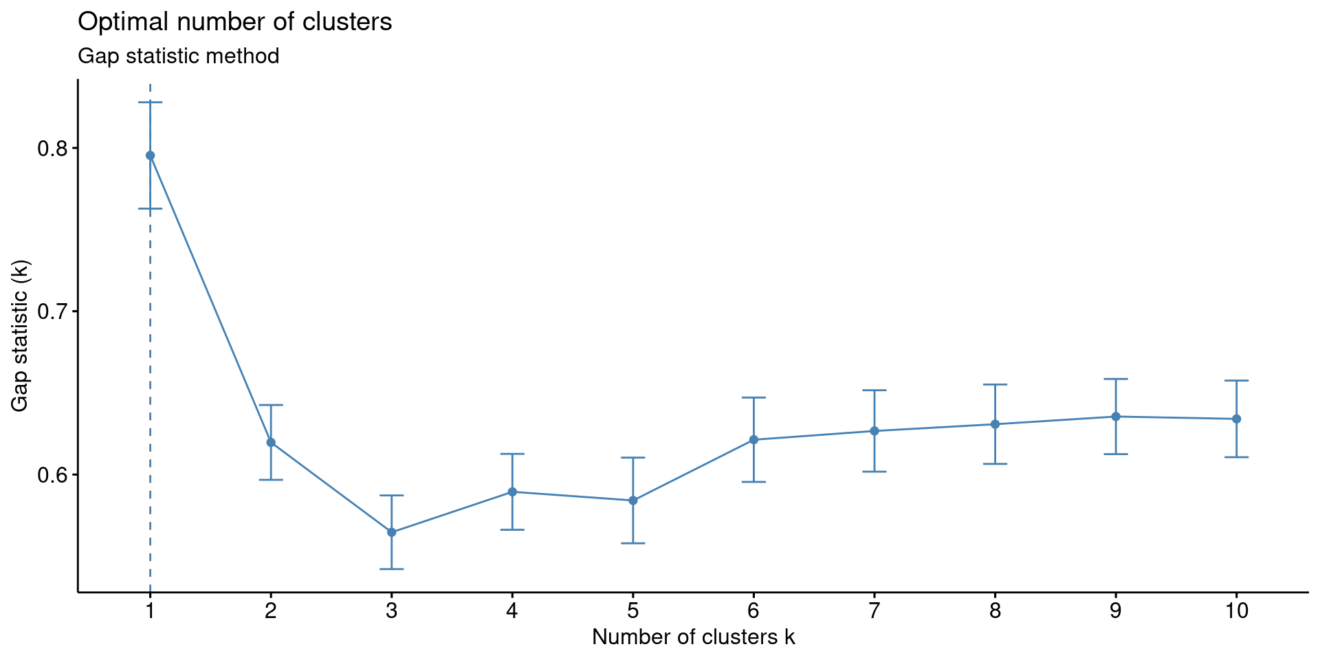
- Gap Statistic Method to identify the optimum number of clusters using a logarithmic function.
- NbClust() uses 30 different methods determine the optimal number of clusters using the “Euclidean” algorithm (Pythagorean Theorem) to find the relative distances between the data points.
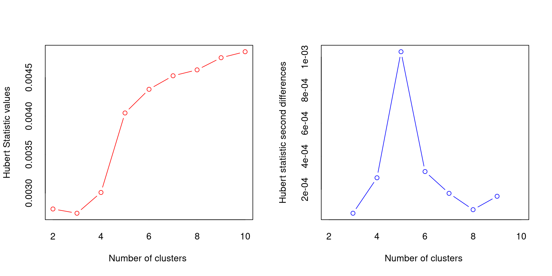
*** : The Hubert index is a graphical method of determining the number of clusters.
                In the plot of Hubert index, we seek a significant knee that corresponds to a
                significant increase of the value of the measure i.e the significant peak in Hubert
                index second differences plot.
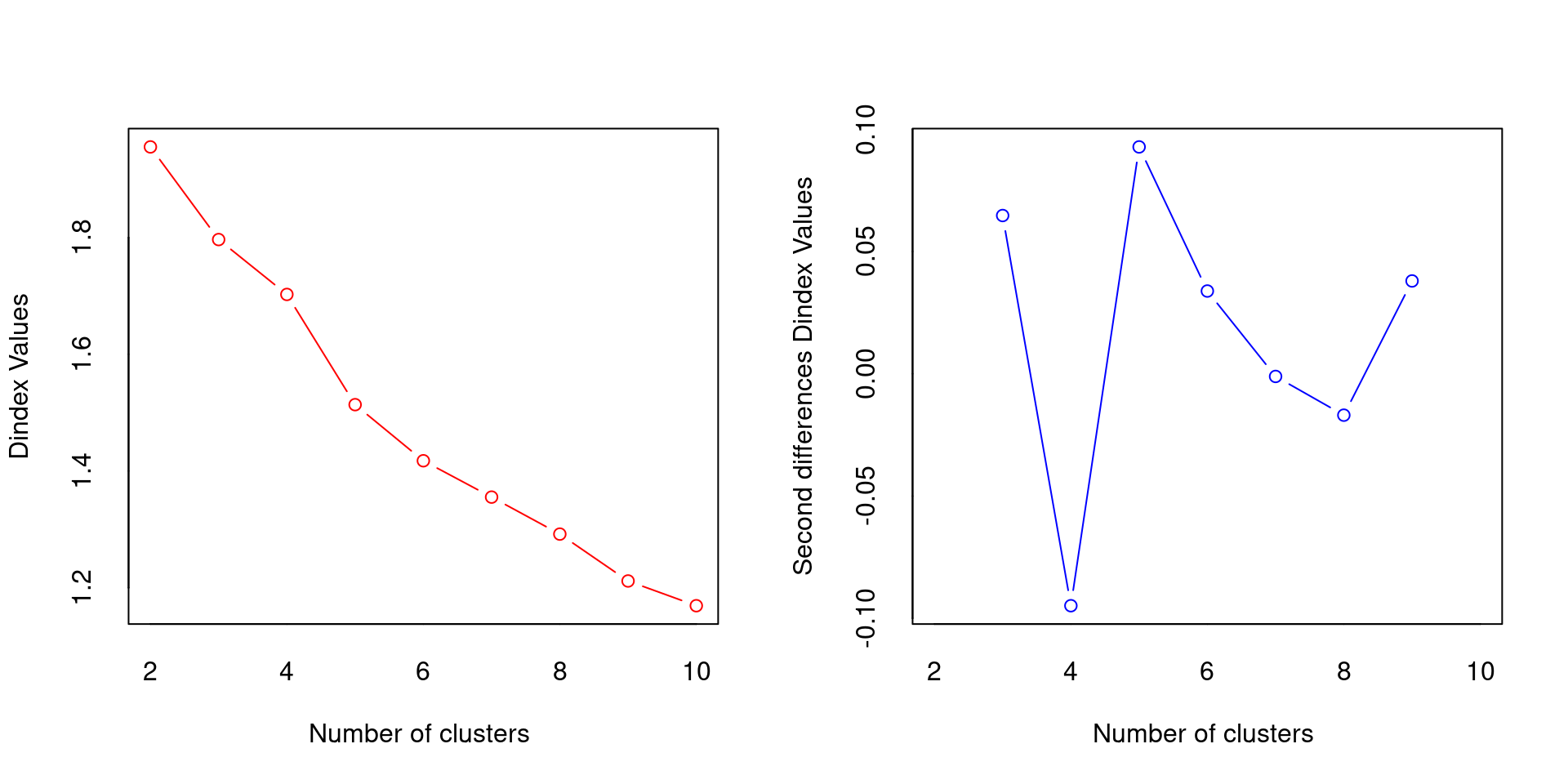
*** : The D index is a graphical method of determining the number of clusters.
                In the plot of D index, we seek a significant knee (the significant peak in Dindex
                second differences plot) that corresponds to a significant increase of the value of
                the measure.

*******************************************************************
* Among all indices:
* 6 proposed 2 as the best number of clusters
* 2 proposed 3 as the best number of clusters
* 3 proposed 4 as the best number of clusters
* 6 proposed 5 as the best number of clusters
* 2 proposed 6 as the best number of clusters
* 1 proposed 7 as the best number of clusters
* 1 proposed 9 as the best number of clusters
* 3 proposed 10 as the best number of clusters

                   ***** Conclusion *****

* According to the majority rule, the best number of clusters is  2


*******************************************************************
Data & Visualization
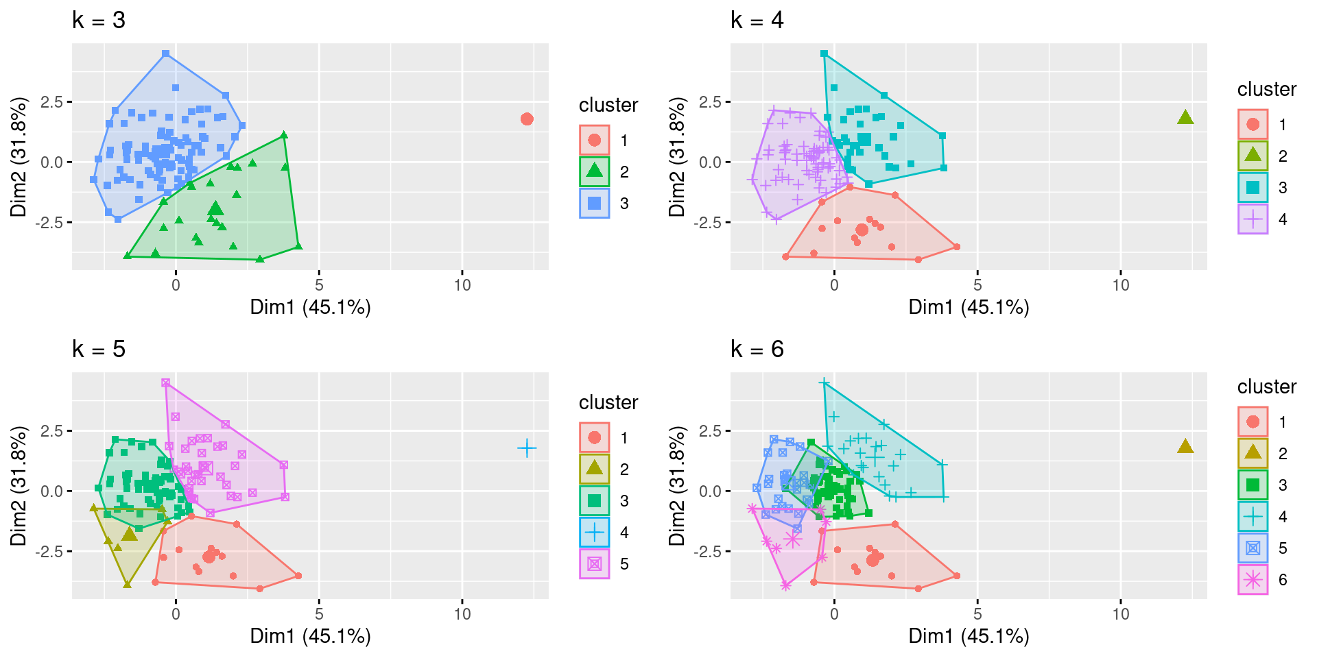
- The coded algorithm fviz_cluster() plots the clusters using the selected number of centroids: k=3 through k=6.